
Deep Learning Based Prepayment Modeling Approach
- ASHISH KUMAR

- Feb 3
- 11 min read

Table of Content
Executive Summary | ||
| ||
| ||
| ||
| ||
| ||
| ||
|
Executive Summary
Accurate forecasting of the Conditional Prepayment Rate (CPR) is critical for precise valuation of Mortgage-Backed Securities (MBS) and effective Asset-Liability Management (ALM). Traditional econometric models, such as Cox Proportional Hazards or Logistic Regression, often struggle to capture the complex, non-linear "tipping points" inherent in borrower prepayment decisions.
This report introduces "DeepPrepay," a novel Deep Neural Network (DNN) architecture designed to overcome these limitations. DeepPrepay uses a multimodal input architecture, incorporating denoising autoencoders to process macroeconomic yield curves and a robust regularization strategy that includes Dropout (Srivastava et al., 2014) and Batch Normalization (Ioffe & Szegedy, 2015).
This advanced methodology excels at capturing characteristic dynamics, such as the "S-curve" of refinancing incentives and the portfolio-specific "burnout" effect. DeepPrepay is built on four key architectural drivers to deliver precise CPR predictions and optimize MBS/ALM strategies:
Tri-Modal Funnel with Autoencoder: Captures non-linear market dynamics.
ELU, Nadam, and Gradient Clipping: Ensures stable convergence even with volatile data.
Batch Normalization and Dropout: Maximizes model generalization.
Embeddings: Effectively resolves high-cardinality geographic risk factors.
1. Problem Description and Justification
1.1 The Business Problem: Predicting Mortgage Prepayment Probability
The primary goal of this project is to develop a predictive model that estimates the probability that a particular mortgage loan will be prepaid in the following month (t+1). Prepayment occurs when a borrower pays off some or all of their outstanding mortgage balance before the scheduled maturity date. This phenomenon introduces Prepayment Risk, the risk that the holder of a mortgage loan or fixed-income security will lose potential future interest payments due to the borrower's early repayment of principal. Voluntary prepayment, often due to refinancing or home sales, introduces "contraction risk" by reducing future interest income and forcing the reinvestment of principal, often at a lower yield when interest rates are falling.
For example, Figure 1 illustrates prepayment risk: a borrower pays off an existing high-interest loan early to capitalize on falling market rates, thereby refinancing to save on interest costs.
Figure 1: Prepayment Risk

Source: WallStreet Mojo
Accurate mortgage prepayment modeling is vital for various stakeholders: lenders use it for risk management, investors in Mortgage-Backed Securities (MBS) rely on it for security valuation, and institutions employ it for capital allocation and hedging.
Outcome Variable (Y):
The predictive model's binary target variable, Y ∈i {0, 1}, indicates prepayment in the next month (Y=1) or no prepayment (Y=0).
1.2 Data Strategy
The proposed model utilizes a heterogeneous dataset mixing structured and unstructured elements to capture a holistic view of borrower intent:
Structured Data
The key factors influencing loan performance can be categorized as follows:
Loan-Specific Characteristics: These include the Current Interest Rate, Original Loan-to-Value (LTV), FICO score, and Loan Age.
Macroeconomic Indicators: Relevant external factors are Treasury Yields, Mortgage Rate Spreads, HPI (House Price Index) growth, and Unemployment figures.
Geographic Data: The Property Location (MSA/ZIP Code) is essential for accurately reflecting regional housing turnover rates.
Unstructured Data:
Behavioral Signals: Deep learning enables the integration of natural language data, such as customer service interaction logs (Goodfellow et al., 2016). These logs often reveal "pre-notification" behaviors in borrowers—such as requesting payoff statements or inquiring about current rates —that precede a formal prepayment request.
The highly dimensional, noisy, and heterogeneous input data (financial metrics, location embeddings, text logs) challenge traditional linear models. These models cannot capture critical nonlinear dynamics (such as the mortgage prepayment "S-curve") or complex latent interactions between textual sentiment and financial indicators, necessitating a deep, hierarchical architecture.
1.3 Limitations of Traditional Linear Models
The Structural Limitations of Traditional Mortgage Prepayment Models
Historically, mortgage prepayment modeling has relied heavily on established statistical techniques, such as the Cox Proportional Hazards model and standard Logistic Regression. These models, by their very design, are semi-parametric and linear, assuming that the probability of a prepayment event can be represented as a simple linear combination of independent, observable variables. While these methods offer interpretability, they are severely limited by structural constraints that fail to capture the complex, nonlinear dynamics (S-Curve) of borrower behavior.
Key Structural Limitations:
Inability to capture “S-curve” in Borrower Behavior
Borrowers' response to interest rate changes is non-linear, following an "S-curve" as they accumulate savings (Figure 2).
Three Stages of Prepayment:
Flat Bottom (Insensitivity): High market rates keep prepayment speeds low; no one refinances.
Steep Middle (Refi Wave): A small rate drop (tipping point) causes a massive surge in refinancing and prepayments.
Flat Top (The Plateau): Further rate declines yield no increase in prepayments as "burnout" occurs; everyone who can refinance has done so.
Figure 2: S-Curve

Source: Gemini
Limitations of Linear Models:
Linear models cannot capture the S-Curve's non-linear patterns. This requires time-consuming, manual feature engineering (e.g., polynomials, interactions, path-dependent look-back variables for "burnout"), which increases model risk.
It wrongly assumes uniform prepayment probabilities for borrowers with the same observable characteristics, ignoring unobserved, borrower-specific behavior (latent heterogeneity). This causes persistent miscalibration, especially during market stress.
Exclusion of Rich, Unstructured Data Sources:
Traditional regression models struggle to process unstructured data, such as free-form text from customer service logs, collection notes, or payment communications, which often contain highly predictive information about borrower risk. These models are limited to structured inputs (numeric and categorical), leaving valuable explanatory power unused.
1.4 Justification for Deep Learning Architecture
Deep Neural Networks (DNNs) surpass traditional linear models by automatically learning complex, non-linear relationships without manual feature engineering. Crucially, a Multi-Modal DNN's flexibility allows it to integrate diverse data, such as structured financial ratios and unstructured text, thereby capturing subtle behavioral and qualitative risk signals that are invisible to purely numerical models. This holistic approach synthesizes disparate streams, detecting nuanced patterns and early signs of distress that linear models miss, significantly boosting prediction accuracy. A shallow Multi-Layer Perceptron (MLP) would fail due to its limited depth for navigating the high-dimensional, multimodal feature space and complex cross-modal interactions, necessitating a DNN for hierarchical abstraction and reliable prediction.
2. Architectural Design using Dense Neural Networks
The architecture employs a hybrid Dense Neural Network (DNN) framework in which a Denoising Autoencoder first compresses complex yield-curve data into robust nonlinear latent features. These encoded signals are then merged with numerical and categorical streams, feeding into a tapering dense "funnel" (e.g., 512→ 64) that progressively distills high-dimensional interactions into precise risk predictions.
2.1 Conceptual Design: Multi‑Layer Perceptron (MLP)
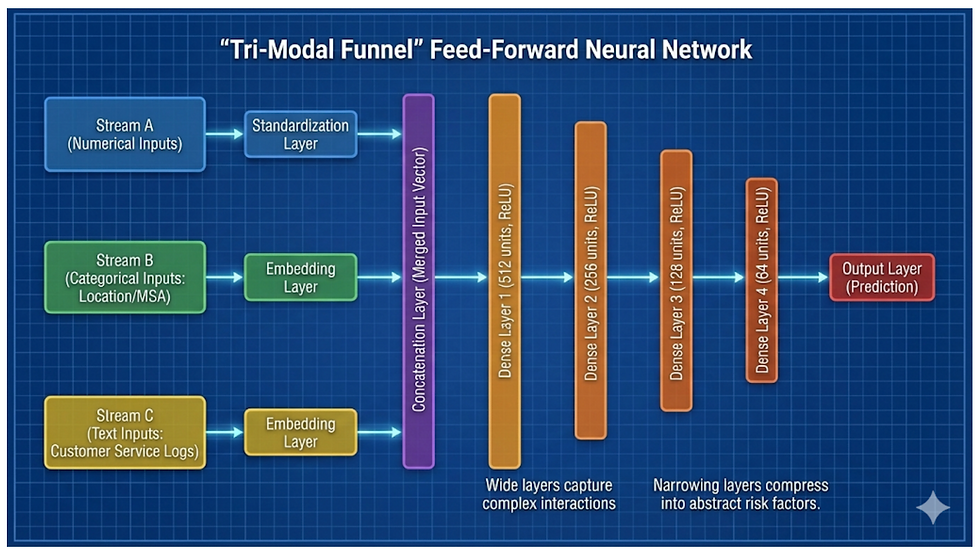
Feed-Forward Neural Network with a "Tri-Modal" input:
Stream A (Numerical): Standardized financial data.
Stream B (Categorical): Location/MSA zip codes mapped to dense vectors.
Stream C (Text): Customer Service Logs converted to "Sentiment/Intent" vectors via an Embedding Layer.
Figure 3 integrates standardized numerical data, location categoricals, and text logs (via embedding/standardization).
A pre-trained, frozen Denoising Autoencoder processes the 15-point Treasury Yield Curve, outputting a 3-dimensional latent vector that feeds into the numerical stream.
These inputs are concatenated into a four-stage, tapering Dense Neural Network (512 to 64 units) that compresses roughly 1,000 features into abstract risk factors, yielding a single scalar risk probability.
Architectural depth (four tapering layers) is prioritized over width to enforce hierarchical feature abstraction, enabling the model to capture complex, higher-order interactions among heterogeneous metrics, macroeconomic trends, geographic embeddings, and text signals that a shallow network would miss.
The final hidden-layer weights transform complex, multimodal features nonlinearly into a single Sigmoid output representing the log-odds of prepayment probability, condensing thousands of interactions.
Figure 3: DNN Architecture
Source: Gemini
2.2 Activation Functions
Hidden Layers: Exponential Linear Unit (ELU). The ELU activation function was selected for the hidden layers, rejecting both the traditional Sigmoid and the standard ReLU functions for specific architectural reasons:
The Sigmoid activation function was abandoned in deep neural networks mainly due to two issues: the Vanishing Gradient Problem and its non-zero-centered output. The bounded output (max derivative 0.25) causes gradients to shrink significantly during backpropagation, slowing learning in early layers. The non-zero-centered output causes "zig-zagging" updates, hindering overall network convergence.
ELU is chosen over ReLU because financial spreads, especially in mortgage finance, are information-dense.
Specifically, a negative spread (e.g., -50 bps) strongly predicts non-prepayment, a signal that ReLU would destroy by clipping to zero. ELU preserves negative values (y = α (e^x - 1)), distinguishing between "zero incentive" and "negative incentive."
Additionally, ELU's negative outputs push the mean activation closer to zero, mimicking Batch Normalization to accelerate learning and improve robust feature extraction (Clevert et al., 2015).
Output Layer: Sigmoid. The Sigmoid function is retained for the final output neuron because, for binary classification, it strictly bounds the output between 0 and 1, representing a valid probability P(y=1).
3. Optimization and Training Strategy
3.1 Gradient Descent and Back-Propagation
Binary classification minimizes prediction error by optimizing the Binary Cross-Entropy (BCE) Loss (the difference between the Sigmoid output layer's probabilities and the actual labels).
The Back-Propagation (BP) algorithm employs the chain rule to compute loss gradients with respect to all weights, utilizing the prediction error.
An optimizer, such as Nadam, iteratively adjusts these weights to minimize error, following a continuous cycle of forward pass, loss computation, and backward pass. We use mini-batch gradient descent with a batch size of 512.
3.2 Fast Convergence: The Nadam Optimizer
The Nadam optimizer was selected over standard Adam, which uses "classical" momentum as explained below.
Nadam Justification:
Nadam employs Nesterov Momentum for "lookahead" gradient calculation, which prevents overshooting the minimum—vital for financial models with sudden changes. This Nesterov component helps maintain velocity over flat areas while effectively slowing near sharp minima, successfully navigating volatile mortgage data.
Consequently, Nadam minimizes oscillations and achieves faster, more robust convergence than Adam on non-stationary financial data.
Learning Rate: To prevent oscillation around the local minima during late-stage convergence, we couple Nadam with a ReduceLROnPlateau scheduler. This hybrid approach allows Nadam to handle feature-specific scaling, while the scheduler enforces global annealing once the validation loss stabilizes.
Batch Size: We employ a mini-batch size of 512, which provides a sufficient sample size to stabilize Batch Normalization statistics while remaining computationally efficient, avoiding the noisy gradients of online learning and the memory constraints of full-batch processing on large mortgage datasets.
Epochs and Early Stopping Strategy:
We prioritize computational efficiency with a generous 100-epoch limit, using Early Stopping based on Validation Loss and AUC as the main controls.
This strategy ensures "fast but safe" convergence by automatically halting training when performance plateaus, capturing optimal weights and preventing overfitting without running redundant epochs.
3.3 Managing Gradient Challenges
Deep financial networks face opposing stability issues during back-propagation. We mitigate these using the Exponential Linear Unit (ELU) and robust clipping.
Vanishing Gradients & The "Dying Neuron" (Solved by ELU): Traditional activations (Sigmoid, ReLU) cause vanishing gradients or "dying neurons" (zero gradients for negative inputs). We use ELU (Clevert et al., 2015). For positive inputs, y = x prevents saturation. For negative inputs, y = ἀ(e^x - 1) maintains a smooth, non-zero gradient, preventing neuron death and ensuring continuous learning.
Exploding Gradients (Managed by Clipping): Financial "fat tails" (outliers) generate large error signals, increasing the risk of weight divergence. Although ELU helps center activations, it does not limit positive outputs. We implement Gradient Norm Clipping (Pascanu et al., 2013). This acts as a "circuit breaker," rescaling the global L2 gradient norm (e.g., 0→1.0) if it exceeds a threshold, preventing market shocks from destabilizing the model.
4. Taming Complexity and Generalization
Training a deep network on volatile mortgage data faces two challenges: Optimization Instability (poor learning) and Overfitting (memorizing noise). We use Batch Normalization and Dropout as a dual-defense strategy to counter both.
4.1 Regularization Techniques
Batch Normalization (BN) handles extreme data and "fat tails". Financial shifts cause Internal Covariate Shift, destabilizing gradients. BN normalizes layer inputs to a standard Gaussian distribution per mini-batch, "dampening" extreme outliers and ensuring a stable signal for faster convergence and higher learning rates.
Dropout prevents overfitting and co-adaptation. Deep networks can memorize specific historical patterns. Dropout randomly sets a percentage of hidden neurons to zero during training (e.g., 30%). This forces the model to develop redundant, distributed risk representations, preventing over-reliance on single features and ensuring robust generalization.
4.2 Ordering Strategy
The architecture uses a "Post-Activation Dropout" topology: Dense → Batch Normalization (BN) → ELU Activation→ Dropout (Figure 4). This order is justified because BN centers the pre-activation input (Dense) for optimal normalization, provides a stable signal to ELU to enable higher learning rates, and Dropout is applied after ELU to mask fully formed features. Applying Dropout before BN is avoided as it would destabilize BN's mini-batch statistics. BN + ELU + Dropout are used after each of the four dense layers in the main funnel, with dropout rates tapering slightly (e.g., 0.3→0.2) as the representation narrows, to reduce overfitting in the early layers while preserving signal in the final layers.
Figure 4: Model Order

Source: Gemini
5. Feature and Data Representation
High-dimensional and high-cardinality features are transformed into dense, meaningful representations for efficient Deep Learning. This involves Denoising Autoencoders for macroeconomic data (e.g., Treasury yields), Entity Embeddings for geographic data (e.g., Zip/MSA), and Word Embeddings for unstructured text (e.g., customer service logs). Standard scaling is used for other low-dimensional numeric features that do not use autoencoders.
5.1 Denoising Autoencoders vs. PCA (Macroeconomic Curves)
To model the Treasury Yield Curve (15+ tenors) despite high multicollinearity, we used a Denoising Autoencoder with a 3-neuron bottleneck, trained with Gaussian noise. This non-linear approach captures complex market dynamics ("twists") more effectively than linear PCA (which only finds Level, Slope, and Curvature), providing a cleaner signal for the prepayment model (Figure 5).
Figure 5: Use of Autoencoder

Source: Gemini
5.2 Categorical Embeddings (Entity Embeddings) for Geography vs. One-Hot Encoding
Standard One-Hot Encoding for the target feature, Property Location (40,000+ Zip Codes), leads to the "Curse of Dimensionality" and sparse vectors, hindering the model's ability to learn shared regional prepayment characteristics. The solution is Learned Entity Embeddings, which map each Zip Code to a small, dense vector (e.g., R10) that is updated via back-propagation. This method automatically clusters Zip Codes with similar prepayment behavior, grouping areas such as San Francisco and New York in the "risk space."
5.3 Word Embeddings vs. Bag-of-Words (Unstructured Text)
Targeting Customer Service Interaction Logs, traditional methods (BoW, TF-IDF) struggle with context and synonymy. The proposed solution uses an Embedding Layer (GloVe/Word2Vec) to create a dense "Context Vector" of borrower intent. This semantic vector, merged with financial and geographic data, helps the main network weigh "Borrower Sentiment" against "Interest Rate Incentive."
Conclusion
DeepPrepay replaces traditional Logistic Regression with a Deep Neural Network for mortgage risk assessment, automatically capturing complex refinancing patterns such as the "S-curve" and "Burnout." Its architecture uses ELU and Gradient Clipping for stability in financial time series, and "Sandwich" regularization (Batch Norm → Activation → Dropout) for fast, robust convergence. DeepPrepay offers a competitive advantage in Asset-Liability Management by leveraging all data, including unstructured text and geographic risk, via Entity Embeddings to provide a holistic view of borrower intent. This sophistication directly leads to superior MBS pricing and better hedging against contraction risk.
References
Clevert, D. A., Unterthiner, T., & Hochreiter, S. (2015). Fast and accurate deep network learning by exponential linear units (ELUs). arXiv preprint arXiv:1511.07289.
Dozat, T. (2016). Incorporating Nesterov momentum into Adam [Conference session]. ICLR 2016 Workshop, San Juan, Puerto Rico.
Goodfellow, I., Bengio, Y., & Courville, A. (2016). Deep learning. MIT Press.
Guo, C., & Berkhahn, F. (2016). Entity embeddings of categorical variables. arXiv preprint arXiv:1604.06737.
He, K., Zhang, X., Ren, S., & Sun, J. (2016). Deep residual learning for image recognition. In Proceedings of the IEEE conference on computer vision and pattern recognition (pp. 770-778).
Ioffe, S., & Szegedy, C. (2015). Batch normalization: Accelerating deep network training by reducing internal covariate shift. arXiv preprint arXiv:1502.03167.
Kingma, D. P., & Ba, J. (2014). Adam: A method for stochastic optimization. arXiv preprint arXiv:1412.6980.
Pascanu, R., Mikolov, T., & Bengio, Y. (2013). On the difficulty of training recurrent neural networks. International conference on machine learning (pp. 1310-1318). PMLR.
Srivastava, N., Hinton, G., Krizhevsky, A., Sutskever, I., & Salakhutdinov, R. (2014). Dropout: A simple way to prevent neural networks from overfitting. The Journal of Machine Learning Research, 15(1), 1929-1958.
About The Author
Ashish (Mehta) Kumar
is a seasoned quantitative professional with 17+ years of experience, blending deep financial industry expertise with strategic consulting insight. His work focuses on applying Generative AI to high-impact financial processes — including documentation summarization, trade settlement automation, model validation, and AI governance — all anchored in Responsible AI principles.
He has worked with leading global institutions in the US such as Moody’s Analytics, S&P Global, and Banco Santander. Since relocating to India in 2020, he has collaborated with organizations like Wells Fargo, HSBC, and EY. Ashish has also spoken at prominent industry platforms including the IndiaAI Responsible AI Mitigation (RAM) Summit and Kore.AI’s Enterprise Conversational AI Forum.
He holds an M.S. in Mathematics from Rutgers University and an M.S. in Engineering from The University of Toledo, USA.


Comments